
Maëlic Neau
RelateAnything
how the things in a picture relate, in words you choose
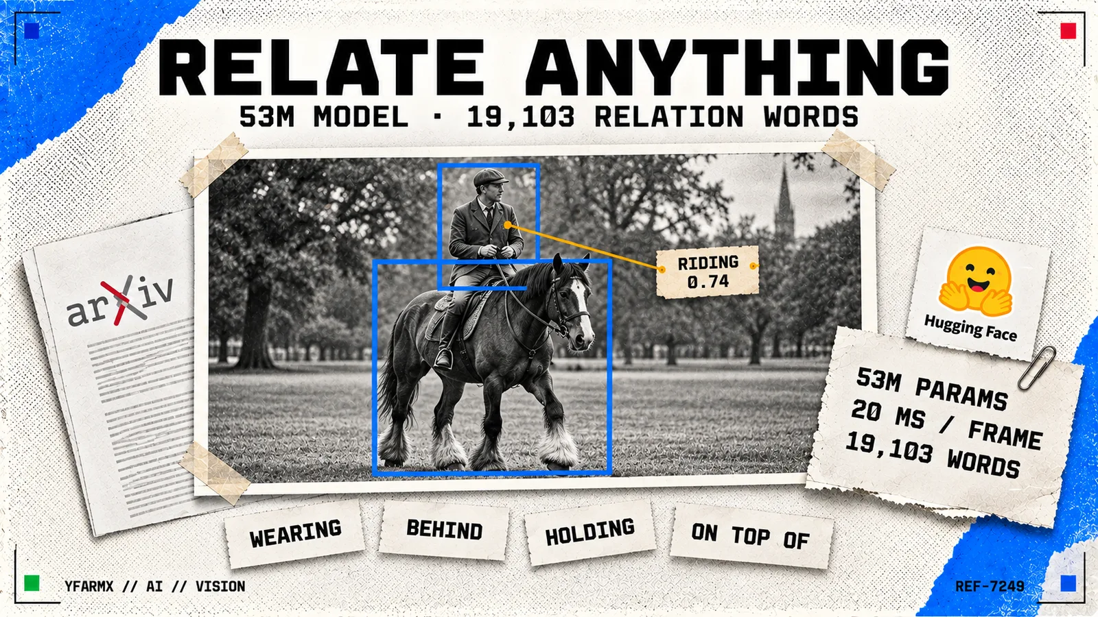
Key facts
- 53MDINOv3 ViT-S/16+
- Parameters
- 20 msa frame on an A40
- Speed
- 19,103relation strings
- Vocabulary
- 0in training or use
- Object labels
Hand it a photo, a set of boxes and your own list of relation words. It scores every pair of boxes against every word in about 20 milliseconds, and it runs in a browser tab.
It reads a picture and says how the things in it relate
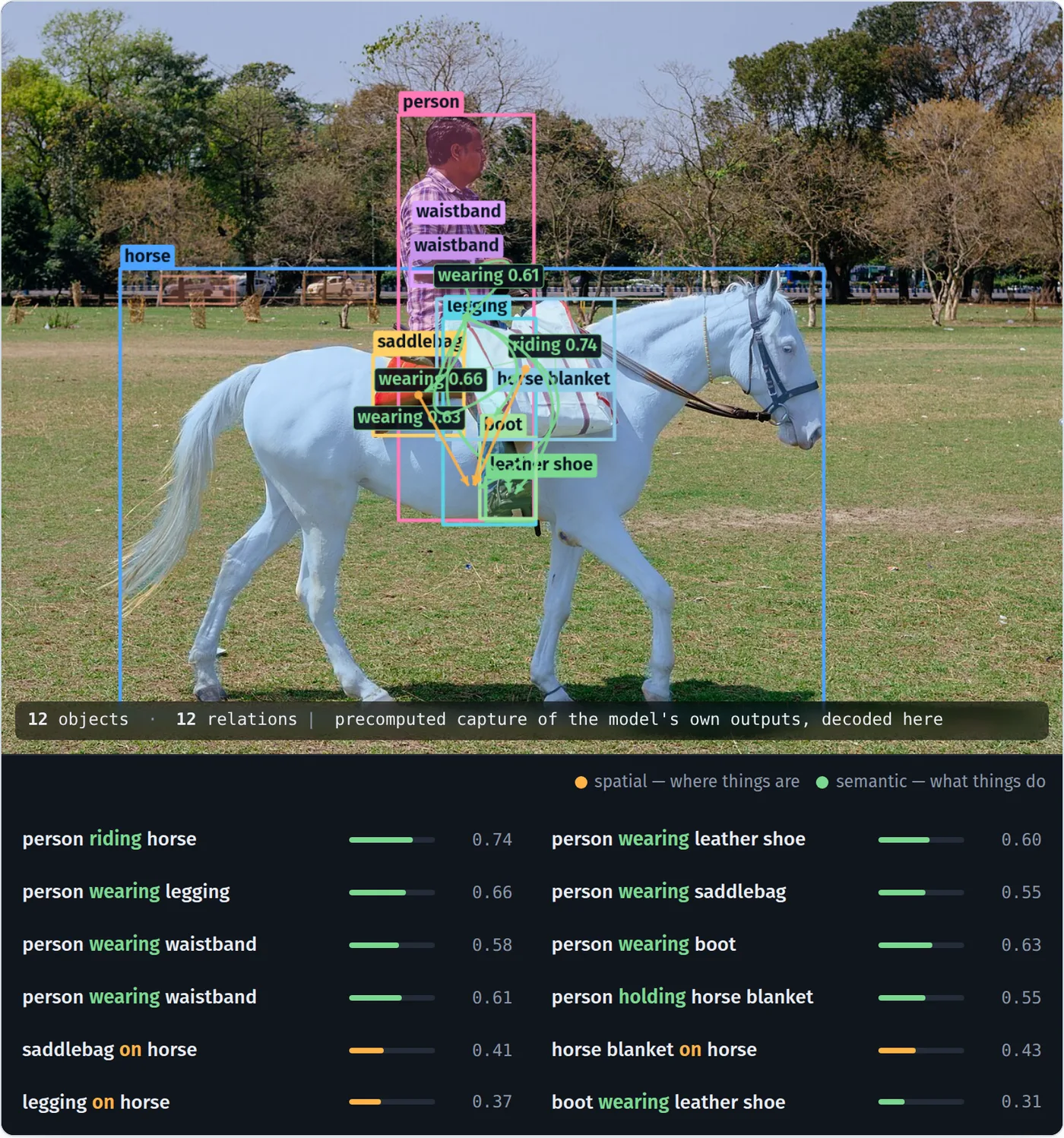
Point a detector at a photograph and you get a list of boxes: a person here, a horse there, a saddlebag, a pair of boots. What the boxes leave open is the sentence that joins them. RelateAnything writes that sentence. Given the image and the boxes, it scores every pair against a list of relation words and returns the ones that hold, with a confidence on each: person riding horse at 0.74, person wearing boot at 0.63, saddlebag on horse at 0.41.
The model is 53 million parameters on a DINOv3 ViT-S/16+ backbone, and it answers in about 20 milliseconds a frame on an A40 including the detector. It was published on 11 September 2026 by Maëlic Neau, working as an independent researcher, with the paper, the weights, the training corpus and the benchmark all released together.
You choose the relation words
The list of relations is an input, not a property of the model. Most scene-graph systems learn one corpus’s fixed set: the standard VG150 benchmark has 50 predicates, and a model trained on it can answer with those 50 and nothing else. RelateAnything can answer with any of the 19,103 strings it was trained across, and it accepts a fresh list at the moment you call it.
That works because the words take a separate path through the model. A distilled 512-dimensional text encoder turns each string into a unit vector, they are stacked into a bank, and no learned layer touches the bank afterwards. Scoring is a cosine between the visual side and the text side. Adding a predicate means adding a row, so a word the model never saw in training is handled exactly like one it did.
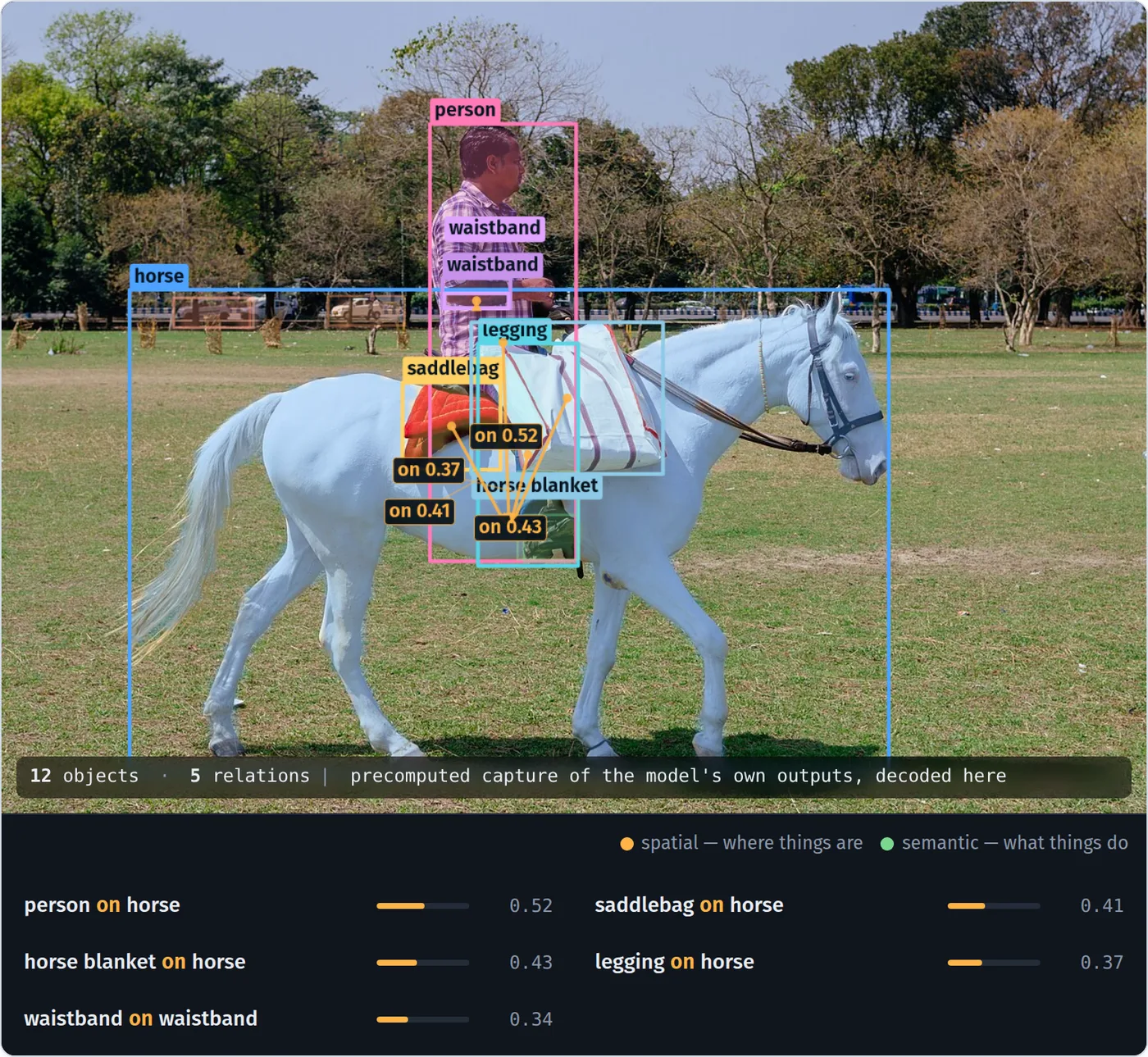
The demo shows the consequence directly. It scores 263 predicate strings against each sample photograph once, then re-runs the decode on those stored scores as you change the word list, so swapping the vocabulary is instant. Its default list of 35 words returns the twelve relations above. Cut that to the 15 spatial words and the same photograph gives a different graph: the riding and wearing edges go, and what survives is person on horse at 0.52, horse blanket on horse at 0.43, saddlebag on horse at 0.41.
It works from pixels and boxes alone
The model is handed the image and the box coordinates. It is given no object class labels, at any point in training or at inference, and the author treats this as the load-bearing design choice rather than a detail.
The standard evaluation protocol hands a model ground-truth boxes together with their classes, which lets it lean on a prior: a person and a bicycle are probably in a riding relation, whatever the pixels say. Neau measures how much of his own model’s answer comes from that kind of prior and reports that 87 to 93 per cent of the semantic score’s variance comes from the pair’s visual context, against 0.1 per cent from object identity. Scoring one image’s boxes against another image’s features costs 44 to 68 per cent of accuracy, which is the check that the pixels are doing the work.
The practical payoff is that the regions can come from anywhere. Any detector will do, and so will a segmenter that produces masks with no class names attached at all. In the demo you can switch the region source from YOLOE, which names objects from 4,585 built-in classes, to FastSAM, which names nothing and returns coloured blobs, and the relation graph is computed the same way.
The training corpus was written by a machine and checked against geometry
Human relation annotation is slow, expensive, and annotators agree with each other poorly. RA-4M, the corpus released alongside the model, takes the other route: an open-weight 26-billion-parameter mixture-of-experts model with 4 billion active parameters annotates images that carry a numbered dot at the centre of each box, in three passes. The whole corpus took 104 GPU-hours.
What makes it usable is the filter that runs afterwards. Deterministic geometric gates reject 11.3 per cent of the raw candidates, and they fire only where box geometry actually constrains the predicate: a contact relation has to touch, containment and proximity are checked against the boxes, and a direction that points the wrong way is repaired by swapping the roles rather than thrown out, with the annotator’s own wording kept. Anything geometry cannot rule on passes through unchecked and is counted as such. Neau states the check as a first: as far as he is aware, RA-4M is the only machine-annotated relation corpus that holds its annotator to box geometry.
The result, measured on the same images and the same boxes as the annotations it replaces:
| RA-4M | source annotations | |
|---|---|---|
| Images | 474,413 | 474,420 |
| Relations | 4,282,531 | 2,510,905 |
| Relations per image | 9.03 | 5.29 |
| Distinct predicates | 10,102 | 94 |
| Predicate entropy | 3.99 nats | 2.56 nats |
Mean object degree rises from 1.88 to 3.20, and the share of images whose graph forms a single connected component goes from 70.9 to 82.6 per cent. The corpus is also direction-balanced by construction: because the annotator prefers the left or upper object as the subject, every verified directional relation is restated from the other endpoint with probability one half, roles swapped and predicate replaced by its inverse.
Ten thousand words, and the top ten still carry 57 per cent
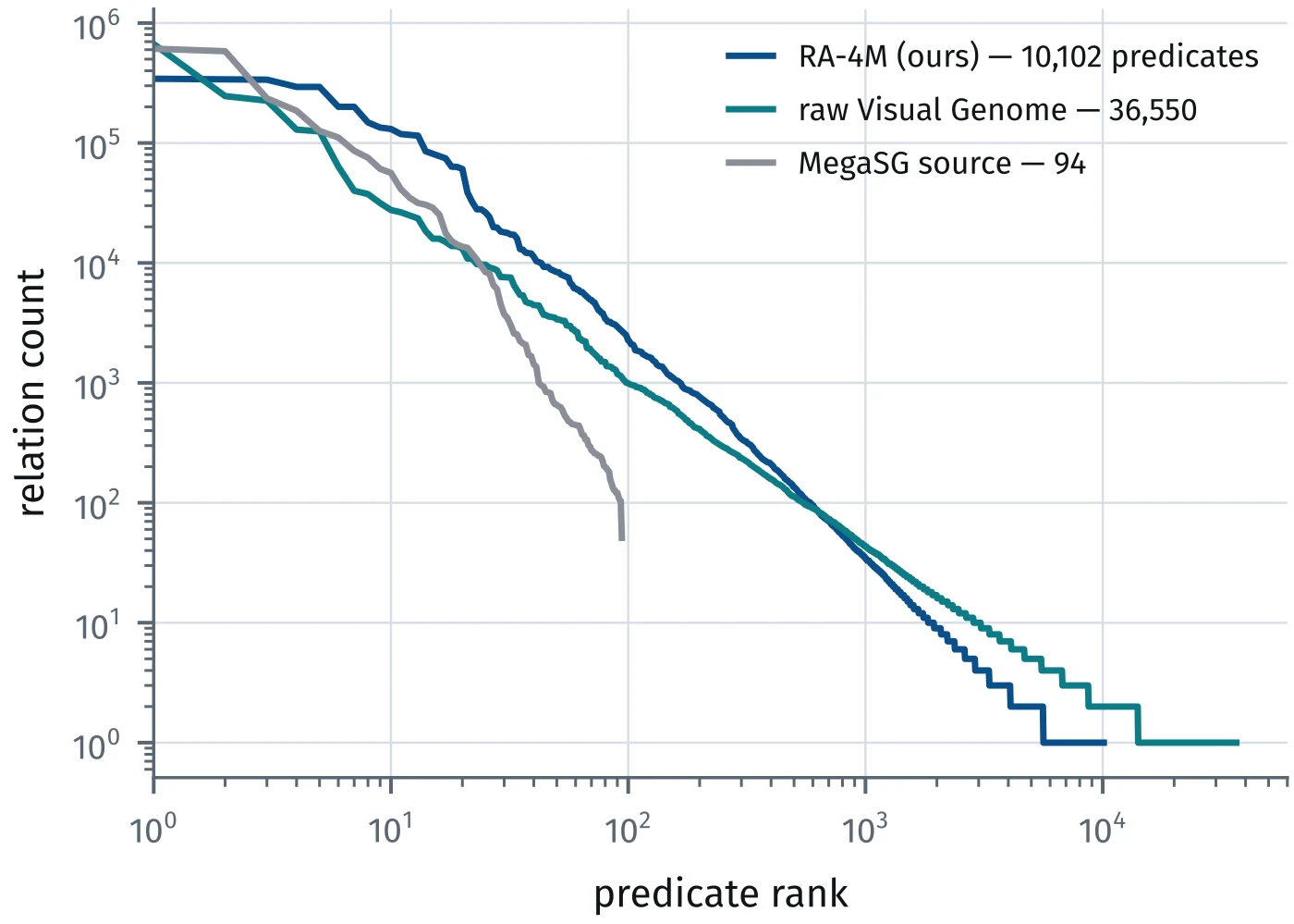
A bigger vocabulary does not spread the weight evenly. In RA-4M the ten most common predicates still account for 57 per cent of all relation instances. What changes is the middle of the distribution: ranks 10 to 100 hold an order of magnitude more relations than the source vocabulary does, and the tail runs out to 10,102 strings where the source stops at 94.
Training across that many predicates changed the loss. With 10,000 words in play, a pair annotated riding is also sitting on and also above, so treating every unannotated predicate as a negative teaches the model to suppress correct answers. Each negative is therefore discounted by the estimated probability that it holds too, fitted on the 706,000 training pairs that carry more than one annotation. Annotated predicates and directional inverses keep their full weight, because separating above from below is the one signal that cannot be softened.
The text encoder had to be rebuilt for the same reason. An off-the-shelf contrastive encoder is direction-blind: it places above and below at cosine 0.95, and the two left/right forms at 0.99, which is indistinguishable from the 0.96 it gives two words that mean the same thing. No visual model regressing onto targets like those can separate them, so the encoder is distilled into a student that pushes inverses apart before the bank is built.
It runs at 20 milliseconds a frame, and inside a browser tab
At batch size one the cost is kernel dispatch rather than parameter count, which is why the faster system here is also the larger one. The baseline scores about 9,500 pairs among 98 boxes at 800 by 1333 in full precision; RelateAnything scores at most 128 sampled pairs among 20 boxes at 448 pixels in half precision. The comparison the author reports, eager PyTorch on both sides and timing the whole system including the detector on an A40:
| System | Parameters | Latency | FPS |
|---|---|---|---|
| RelateAnything + YOLO-World | 231M | 25.0 ms | 40.0 |
| OvSGTR Swin-T | 177M | 194.0 ms | 5.1 |
| OvSGTR Swin-B | 237M | 228.5 ms | 4.3 |
Compiled, the model reaches 20.3 ms and 49 FPS on an A40, and 18.1 ms on an H100. On eight CPU threads through OpenVINO it manages 7 FPS while agreeing with the full-precision run on 95.5 per cent of top-1 predictions. Scoring all 19,103 strings rather than 50 costs under a millisecond, because the predicate bank is an input tensor to a single ONNX graph rather than something baked into the export.
That last property is what puts it in a browser. The demo downloads about 105 MB for the model and 5 to 27 MB per detector, then caches both; the relation head takes roughly 600 ms per frame under WebAssembly and the detector 80 to 500 ms. Weights are stored at half precision and computed at full, which halves the download and runs on both of ONNX Runtime Web’s providers. Calibration is two floats, taking expected calibration error from 0.176 to 0.004, so the confidence numbers on screen are meant to be read as probabilities.
How it scores against the other systems
The release ships its own benchmark, OV-SGG-Bench, which reports six axes: transfer, precision against adjudicated negatives, open vocabulary, deployment on a shared detector, graph quality judged by a vision-language model, and spatial relations. The chance-corrected composite across five of them is 40.1 for RelateAnything against 11.8 for OvSGTR, the strongest open-vocabulary baseline of comparable scale, and the baseline is given ground-truth object labels while RelateAnything is not.
Across three benchmarks that contributed no training image and a fourth scored zero-shot, the headline margins are 2.3 to 3.5 times the baseline’s mean recall, 5 to 21 times its rare-predicate recall, and 7.8 times the speed.
Deployed with the full 19,103-string vocabulary and synonym-tolerant matching, the correct relation is the model’s median first choice on two of the three benchmarks, ranking 1 of 19,103 on VG150 and IndoorVG and 10 of 19,103 on PSG.
| Benchmark | R@50 | mR@50 | Median rank |
|---|---|---|---|
| VG150 | 56.0 | 34.5 | 1 / 19,103 |
| PSG | 30.5 | 28.3 | 10 / 19,103 |
| IndoorVG | 53.3 | 34.6 | 1 / 19,103 |
Recall on the rare predicates specifically, the part of the distribution a fixed 50-word head has the least of, runs 39.6 on VG150, 34.6 on IndoorVG and 20.8 on PSG.
Against ROBIN-3B, a scene-graph model built on a 3-billion-parameter vision-language model, RelateAnything leads on both recall metrics on all three benchmarks the two were run on, at under 2 per cent of the parameters. How the scoring is done decides part of that. On PSG mean recall ROBIN is ahead under exact-string matching, 20.0 against 13.0, and RelateAnything is ahead under every synonym-tolerant matcher, 31.3 against 25.1. Exact matching penalises hardest the system answering from 19,103 strings, so it is worth 23.2 recall points to RelateAnything and 11.7 to ROBIN, which is a larger swing than the gap it is being used to measure.
The figure that survives every scoring convention is pairs reached, the share of annotated object pairs a system names at all: 99.7 per cent for RelateAnything, 45.6 to 77.4 per cent for ROBIN depending on the matcher, and 23.1 to 35.5 per cent for general multimodal models prompted for the same output. A relation can only be scored right on a pair the system actually names.
A lookup table beats it on the metric the leaderboards use
The most useful thing in the release is the part that undercuts its own numbers. Neau builds a frequency baseline that looks up the most common training predicate for a given subject-object category pair. It reads the ground-truth object labels, and it never sees the image at all. On per-edge accuracy it wins on all three benchmarks, scoring 68.4 against RelateAnything’s 57.7 on VG150. On the per-predicate average of the very same predictions it loses, 18.9 against 35.1.
His conclusion is that a metric a lookup table can win is measuring corpus agreement rather than relation understanding, and it is the metric leaderboards are ordered by. Three further findings run the same way:
- Shared triplet mass is the confound, and it is rarely reported. Two corpora can use the same predicate string and never assert it of the same pair of object categories. Measured as whole triples, the baseline’s fine-tuning corpus overlaps VG150 by 90.9 per cent; RelateAnything’s training mixture overlaps it by 12.8 per cent.
- Two scoring conventions move results more than the methods do. The standard detection-mode matcher has no assignment constraint, so a ground-truth object covered by several detections gives several chances at the same relation, a mean of 2.99 on VG150 test. Adding the constraint costs the baseline 2.45 recall points; upgrading its backbone from Swin-T to Swin-B is worth 2.39. Separately, moving only the detector’s confidence threshold and box cap shifts the achievable ceiling by 19 points, where the spread between all published methods on that leaderboard is 4.3.
- In-domain measurement overstates transfer by roughly five times. Doubling the training corpus is worth 15 per cent micro and 56 per cent macro recall on the corpus’s own validation split, and 2.5 to 3.8 per cent and 9.9 to 11.9 per cent on benchmarks the model never trained on. One design choice changes sign outright between the two readings.
Acting on that last one, the author stopped generating data: the extrapolated gain from another 500,000 annotated images came to about one point, so they were left ungenerated. An audited Open Images extension of 62,589 images, mixed in at a deliberately amplified 25 per cent share, came out negative on every axis, about 6 per cent down on the development composite and 40.2 per cent down on its worst cell, because at 4.33 relations per image its unannotated pairs enter training as false negatives.
Spatial words are the weakest part
The spatial axis is where the release is most candid about its own ceiling. On SpatialSense, an adversarial set with balanced true and false predicates where knowing that on is common buys nothing, RelateAnything reaches 69.0 macro AUC against the baseline’s 59.1. Within that, on and in are learned; above, to the left of and next to sit at chance, and the author reports that fifteen months of recipe changes did not move them.
Neau then refuses his own headline figure. SpatialSense’s original authors built a baseline that reads the boxes and never sees the image, and it scores 68.8. Run under that comparison, RelateAnything reaches 62.5 and the baseline 59.0, so a system working from box coordinates alone stays ahead of both. He draws the conclusion himself in the results notes: an AUC near 0.69 falls short of evidence for visual spatial reasoning, and this stays the release’s weakest axis.
Two other limits are stated in the paper. Gaze is the largest class the geometric filter cannot check, and about 22 per cent of looking at and watching annotations in the corpus have boxes that do not overlap. And in detection mode the ceiling is set by the detector’s operating point more than by the relation model, which is the same finding as the box-cap result above, seen from the deployment side.
What you can download, and the licences on each piece
Three checkpoints are published, all on DINOv3 backbones:
| Checkpoint | Backbone | Parameters | Latency (A40) |
|---|---|---|---|
| relsgg-vits16 | ViT-S/16 | 46.1M | 19.5 ms |
| relsgg-vits16plus | ViT-S/16+ | 53.2M | 20.0 ms |
| relsgg-vitb16 | ViT-B/16 | 113.8M | 19.3 ms |
The middle one is the default, and the one every headline figure on this page refers to. Usage is three lines of Python: load from the Hugging Face hub, hand predict an image and an array of boxes, and optionally call set_vocabulary with your own list of strings first.
The licensing is layered, and the corpus is the piece to read first. The code and the demo are Apache-2.0. The weights derive from Meta’s DINOv3 and carry the DINOv3 licence. RA-4M itself is CC BY-NC 4.0, so the annotations are for non-commercial research use; they were generated by a Gemma model and carry the Gemma terms of use as well, and the images underneath come from Objects365 (56.9 per cent), Open Images V6 (37.6 per cent) and COCO (5.5 per cent), each still governed by its own corpus terms. The demo’s detectors are Ultralytics exports under AGPL-3.0, its text encoder is under Apple’s MobileCLIP licence, and its sample photographs are Creative Commons images from Wikimedia Commons.
Worth noting where the sources disagree: the repository’s third-party notices name only the Gemma terms on the annotations, while the dataset card on Hugging Face carries CC BY-NC 4.0 in its metadata and states it in prose. The dataset card is the stricter of the two, and it is the one attached to the files you download.
The paper itself is arXiv 2609.12552, released under CC BY-SA 4.0.
More in Robotics
All Robotics →- Machine vision and SLAMhow a robot knows where it is
- Embodied AIintelligence with something to lose
- Robot foundation modelsone brain, many bodies
- Humanoid robotsthe human template, and why every lab is copying it
- Industrial robots and cobotsthe five million machines already at work
- Warehouse automationwhere robots already outnumber the pilots